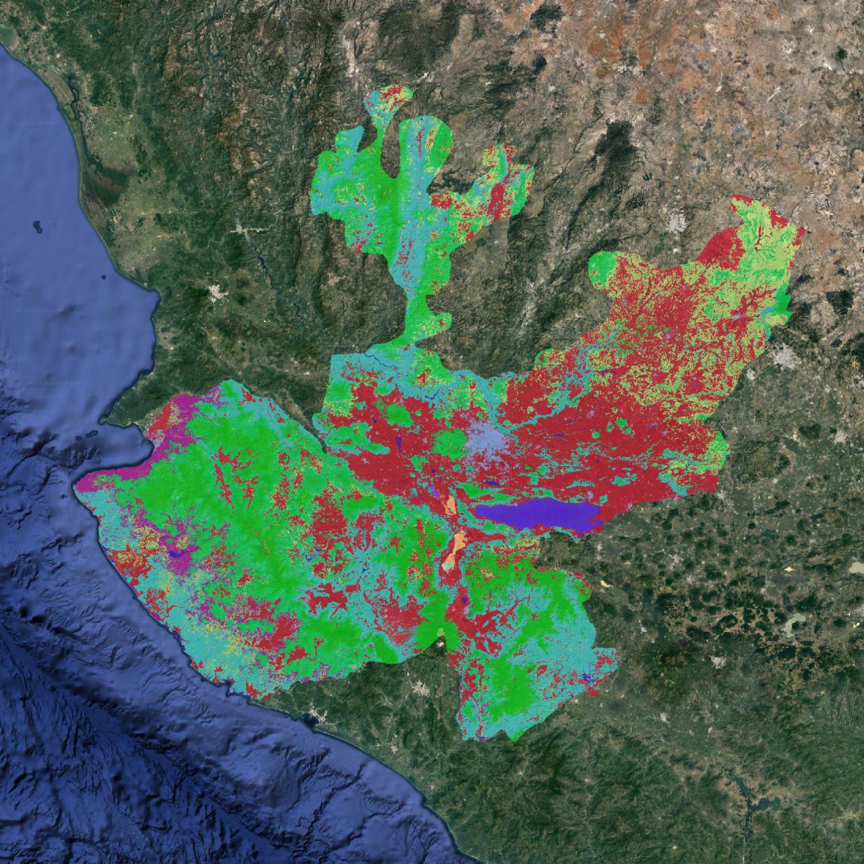
Sentinel 2 based Land cover example
The following example details the step to produce a Land cover map of the state of Jalisco based on Sentinel 2 data at 20 meters resolution.
Datasets preparation
The process of creating a land cover map requires several input that have to be prepared prior to starting the process. These include:
Training data in vector format
Full state coverage of a complete year of sentinel 2 data processed to L2A level (bottom of atmosphere refectance)
Full state coverage of the SRTM digital elevation model with terrain metrics computed.
Ingestion of training data
TODO
Note that contrary to the present example, training data do not need to be a complete coverage of the area to classify.
Download Sentinel 2 L1C data
TODO
Process Sentinel 2 data to L2A level
Note that this was done externally using this docker image for antares does not have a pre-processing module at the moment, however we plan to provide functionalities directly integrated into antares in the future to perform this type of operations. Also note that ESA is planning to process the data themselves to level 2A, so that this step will not longer be required in the future.
Prepare terrain metrics
Before ingesting the elevation data in the datacube, terrain metrics have to be computed. That step is done outside of antares, using gdal’s terrain utilities.
The following lines, ran directly on the compressed SRTM tiles, enable creation of an elevation mosaic and derive slope and aspect from it.
file_list=$(ls *zip|sed -n 's/\(.*\).zip/\/vsizip\/\1.zip\/\1.tif/g;p'|tr -s '\n' ' ')
gdal_merge.py -o srtm_mosaic.tif $file_list
gdaldem slope srtm_mosaic.tif slope_mosaic.tif -s 111120
gdaldem aspect srtm_mosaic.tif aspect_mosaic.tif
Ingest terrain metrics
The process described below consists in ingesting previously generated terrain metrics (elevation, slope, aspect) in the datacube. The process can be divided in two step; first the data are indexed, meaning that a reference to the original GeoTiff files is registered in the datacube database, and second the data are ingested, meaning that the data are resampled to a user defined regular grid, and written to datacube storage units (netcdf or s3 depending on the type of deployment you chose).
# Create product from a product description configuration files
datacube -v product add ~/.config/madmex/indexing/srtm_cgiar.yaml
# Index mosaic
antares prepare_metadata --path /path/to/dir/containing/srtm_terrain_metrics --dataset_name srtm_cgiar --outfile ~/metadata_srtm.yaml
datacube -v dataset add ~/metadata_srtm.yaml
datacube ingest -c ~/.config/madmex/ingestion/srtm_cgiar_mexico.yaml --executor multiproc 10
The two products (indexed and ingested) should now be present in the datacube product list.
datacube product list
Ingest Sentinel 2 bottom of atmosphere data into the datacube
Similarly to the digital elevation model, sentinel 2 data have to be indexed in the datacube database and ingested into a user defined regular grid. These steps are done using the following commands.
# Create product from a product description configuration files
datacube -v product add ~/.config/madmex/indexing/s2_l2a_20m_granule.yaml
# Index the granules
antares prepare_metadata --path /path/to/s2/L2A/data --dataset_name s2_l2a_20m --outfile ~/metadata_s2.yaml
datacube -v dataset add ~/metadata_s2.yaml
datacube ingest -c ~/.config/madmex/ingestion/s2_l2a_20m_mexico.yaml --executor multiproc 10
Generate intermediary product
An intermediary product is a product that contains carefully selected and computed features later used to build a land cover prediction model. Intermediary products are built by applying a recipe to an ingested product over a user defined time range. The recipe we are using in the present example is called s2_20m_001. It computes over a given time range the temporal mean of each sentinel 2 spectral band, the temporal mean, max and min of NDVI and NDMI, and combine these features with the terrain metrics available. The intermediary product generated by applying this recipe therefore contain the following features: blue_mean, green_mean, red_mean, re1_mean, re2_mean, re3_mean, nir_mean, swir1_mean, swir2_mean, ndvi_mean, ndmi_mean, ndvi_min, ndmi_min, ndvi_max, ndmi_max, elevation, slope and aspect.
To generate the intermediary product from the recipe, run the command below. It will be registered in the datacube list of products under the name s2_001_jalisco_2017_0.
antares apply_recipe -recipe s2_20m_001 -b 2017-01-01 -e 2017-12-31 -region Jalisco \
    --name s2_001_jalisco_2017_0
The intermediary product generated will be used in all subsequent stages of the map generation.
Run spatial segmentation
The final map is composed of spatial objects, also called segments. A spatial segmentation step is therefore required.
antares implements various segmentation algorithms that can all be operated from the antares segment command line. To get a list of implemented algorithms, run the antares segment_params command line.
We will use the Berkeley Image Segmentation (bis) for the present example. Each algorithm has different parameters, that can be inspected using the antares segment_params 'algorithm' command line.
Experimenting with the data, we found t=40, s=0.5 and c=0.7 to be an appropriate set of segmentation parameters for this dataset. We can therefore start the segmentation using the following command. Also the command line allow to select a subset of layers to run the segmentation. In this case we choose to use green_mean, red_mean, nir_mean, swir1_mean, swir2_mean, ndvi_mean and ndmi_mean.
antares segment --algorithm bis -n s2_001_jalisco_2017 -p s2_001_jalisco_2017_0 -r Jalisco \
    -b green_mean red_mean nir_mean swir1_mean swir2_mean ndvi_mean ndmi_mean \
    --datasource sentinel_2 --year 2017 -extra t=40 s=0.5 c=0.7
At the end of the process (about 1 hour using 20 parallel processes), you should see the following message informing you of the amount of tiles processed.
Successfully ran segmentation on 19 tiles
0 tiles failed
The resulting segmentation should now appear in the list of segmentation returned by the antares list segmentations command line.
antares list segmentations
name                                              algorithm
---------------------                             ---------------------
s2_001_jalisco_2017                               bis
landsat_bis_test_2017                             bis
landsat_slic_test_2017                            slic
Train the a model
Training a model consists in defining the signature of each land cover class so that it can be recognized and the class be assigned properly in the prediction step. For that, training polygons ingested at the beginning of this example are overlayed with the intermediary product and overlapping areas are extracted, spatially averaged, prepared to be used as training samples and fed to a model (training samples are combined across tiles, so that a single model is trained for the entire area). Once the model has been trained, it is saved on disk and indexed in the antares database.
Similarly to segmentation algorithms, antares offers an interface to various prediction models. To get a list of the models implemented, one can run antares model_params.
The following example uses the random forest decision tree model, which parameters can be consulted using antares model_params rf.
Without much justification, we will build a model composed of 100 trees with a maximum depth of 20. Note that by default 20 percents of the training polygons is selected for training, this value can be adjusted using the -sample command line argument.
antares model_fit -model rf -p s2_001_jalisco_2017_0 -t jalisco_chips --region Jalisco \
    --name rf_s2_001_jalisco_2017 -sp mean -extra n_estimators=100 max_depth=20
Once the command complete, there must be a new prediction model registered in the database. The list of registered models can be consulted using the antares list models.
Predict land cover class
The prediction step uses the previously trained model to predict the land cover class of each polygon generated by the segmentation step. That step is operated with the antares model_predict_object command line.
antares model_predict_object -p s2_001_jalisco_2017_0 -m rf_s2_001_jalisco_2017 \
    -s s2_001_jalisco_2017 -r Jalisco --name s2_001_jalisco_2017_bis_rf_0
Note that the same model can be used to predict land cover class over several time ranges.
Export and visualize the result
If you do not have a web-service to directly visualize the results of the classification from the database, you can export them to a vector file using the antares db_to_vector command line and visualize them in your favorite GIS software.